TL;DR: This tutorial shows how to process 5G RAN telemetry from OpenTelemetry Collectors through GlassFlow (deduplication + schema normalization) into ClickHouse for real-time signal quality analytics using a real-world dataset of 188,711 measurements across 274 cells.

Modern 5G networks generate an enormous volume of telemetry. Every cell continuously reports signal-quality indicators such as Reference Signal Received Power (RSRP), Reference Signal Received Quality (RSRQ), Signal-to-Noise Ratio (SNR), and throughput measurements that operators use to monitor network health. These metrics power everything from SLA reporting and capacity planning to anomaly detection and troubleshooting degraded user experiences.

The challenge is that telemetry rarely arrives as a single clean stream.

Large telecom deployments often use redundant OpenTelemetry Collectors to improve reliability, but this can result in duplicate metric emissions reaching the analytics backend. At the same time, multi-vendor environments introduce inconsistent attribute naming, while synthetic health checks add operational noise. Together, these issues can distort the telemetry operators rely on.

For radio access network (RAN) monitoring, the impact is significant. Duplicate measurements can inflate counts and skew throughput calculations, making it harder to accurately identify signal degradation, capacity issues, and other network problems.

In this article, we'll build an end-to-end pipeline that ingests 5G signal-quality metrics through OpenTelemetry, processes them with GlassFlow, and stores the cleaned stream in ClickHouse for real-time analytics.

GlassFlow is a stream processing platform that sits between your telemetry sources and analytics backends. It accepts OTLP metrics natively and lets you apply transformations (deduplication, filtering, schema normalization) before data reaches storage. Check our open source repository here.

Using a real-world 5G dataset containing nearly 189,000 measurements across 274 cells, we'll simulate a production-style collector topology and demonstrate how GlassFlow can:

• Deduplicate overlapping metric emissions from redundant collectors

• Normalize vendor-specific attribute schemas into a canonical format

• Filter synthetic health-check traffic before it reaches storage

• Deliver clean, trustworthy telemetry to ClickHouse with sub-minute latency

The result is a per-cell observability dashboard that highlights genuine signal degradation trends without double-counting metrics or forcing expensive cleanup operations inside the database.

What you’ll learn

By the end of this article, you will know how to:

• Remove duplicate metric emissions from redundant OpenTelemetry Collectors

• Normalize vendor-specific attribute schemas using GlassFlow stateless transforms

• Filter health-check noise from your telemetry stream

• Store clean, analysis-ready metrics in ClickHouse using a simple MergeTree table

• Detect signal degradation events with ClickHouse SQL queries

Why OpenTelemetry Alone Doesn't Solve This

OpenTelemetry makes it easy to collect and transport telemetry, but it doesn't guarantee that the data arriving at your analytics platform is clean (check out the figure below).

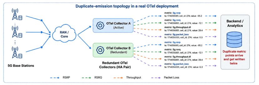
Figure 1. Redundant OpenTelemetry Collectors forwarding identical RAN telemetry to downstream analytics systems.

In telecom environments, redundant OpenTelemetry Collectors are commonly deployed to prevent data loss. The same 5G signal-quality measurement can be forwarded by multiple collectors, creating duplicate records downstream. For metrics such as RSRP, RSRQ, SNR, and throughput, these duplicates can distort aggregations, dashboards, and SLA reporting.

There's also the challenge of consistency. Different network vendors often use different attribute names for the same entities, making cross-network analysis more difficult than it should be.

These issues aren't unique to the telecommunications industry. They're common in large observability deployments. OpenTelemetry standardizes telemetry collection, but tasks such as deduplication, schema normalization, and noise filtering still need to happen somewhere in the pipeline.

In this article, we'll clean the telemetry stream before it reaches ClickHouse using GlassFlow, ensuring that downstream analytics are built on accurate and consistent data.

The Architecture: OpenTelemetry → GlassFlow → ClickHouse

For this demo, we'll simulate a fleet of 5G cells continuously reporting signal-quality metrics such as RSRP, RSRQ, SNR, and throughput. The telemetry is exported through two OpenTelemetry Collectors configured as a high-availability pair, mirroring the redundant collector topologies commonly used in production environments.

Both collectors forward metrics to GlassFlow using the OpenTelemetry Protocol (OTLP). Rather than storing the data immediately, GlassFlow processes the stream first, removing duplicate observations, filtering unwanted telemetry, and standardizing attributes into a consistent schema.

Behind the Scenes: How GlassFlow Processes OTLP Metrics

When OTLP metrics arrive, GlassFlow converts each metric data point into a stream record that can be processed by transformations. The pipeline we'll build applies four operations in sequence:

1. Create a deduplication key from the metric identity.

2. Remove duplicate observations arriving from redundant collectors.

3. Filter health-check telemetry that adds noise but no analytical value.

4. Normalize vendor-specific attributes into a common schema.

The final result is a clean stream of per-cell metrics that can be written directly into ClickHouse for analytics.

Once the stream has been cleaned, the resulting records are written to ClickHouse, where they can be queried in near real time and visualized through Grafana dashboards.

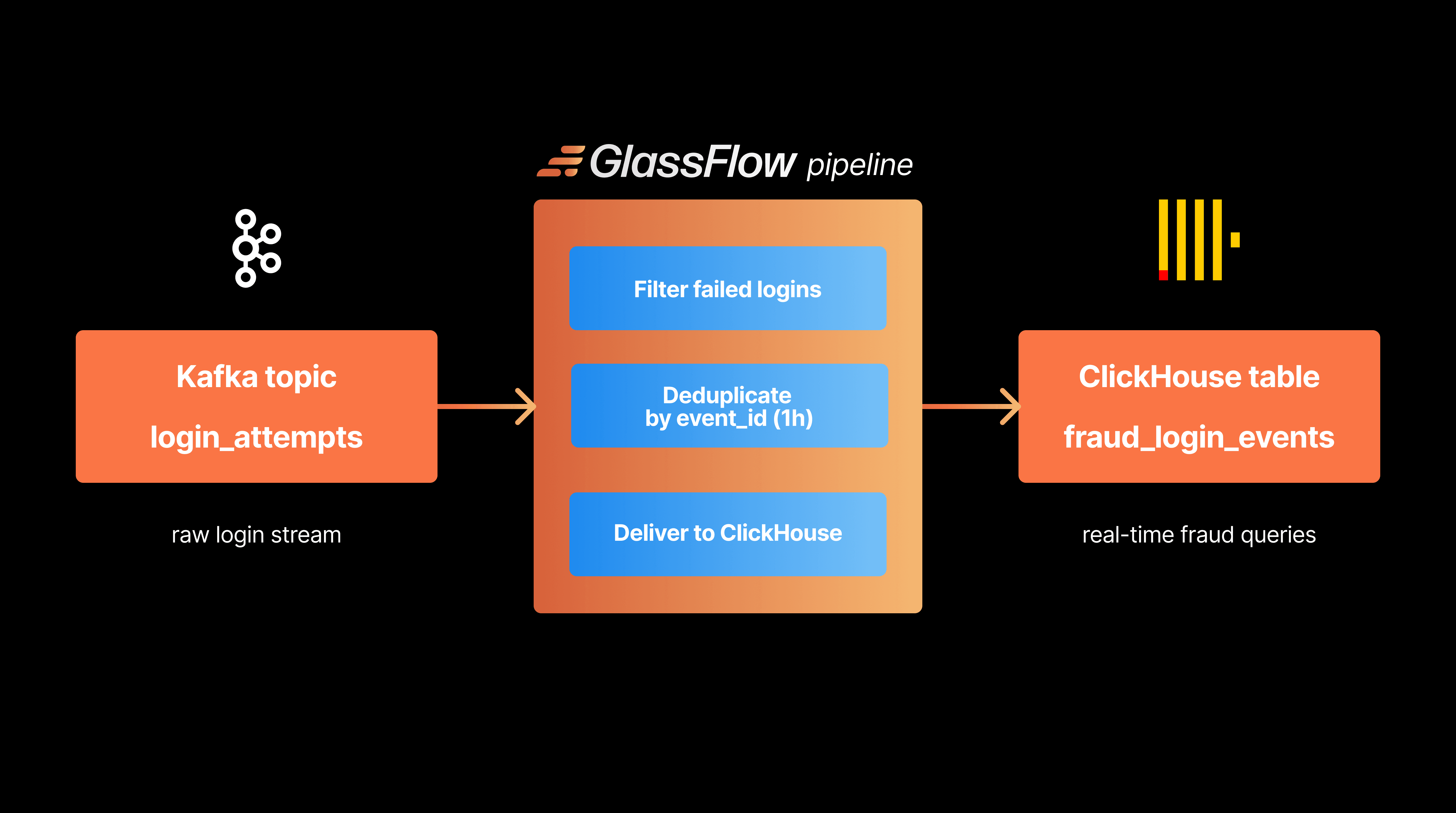
The resulting architecture will be as follows:

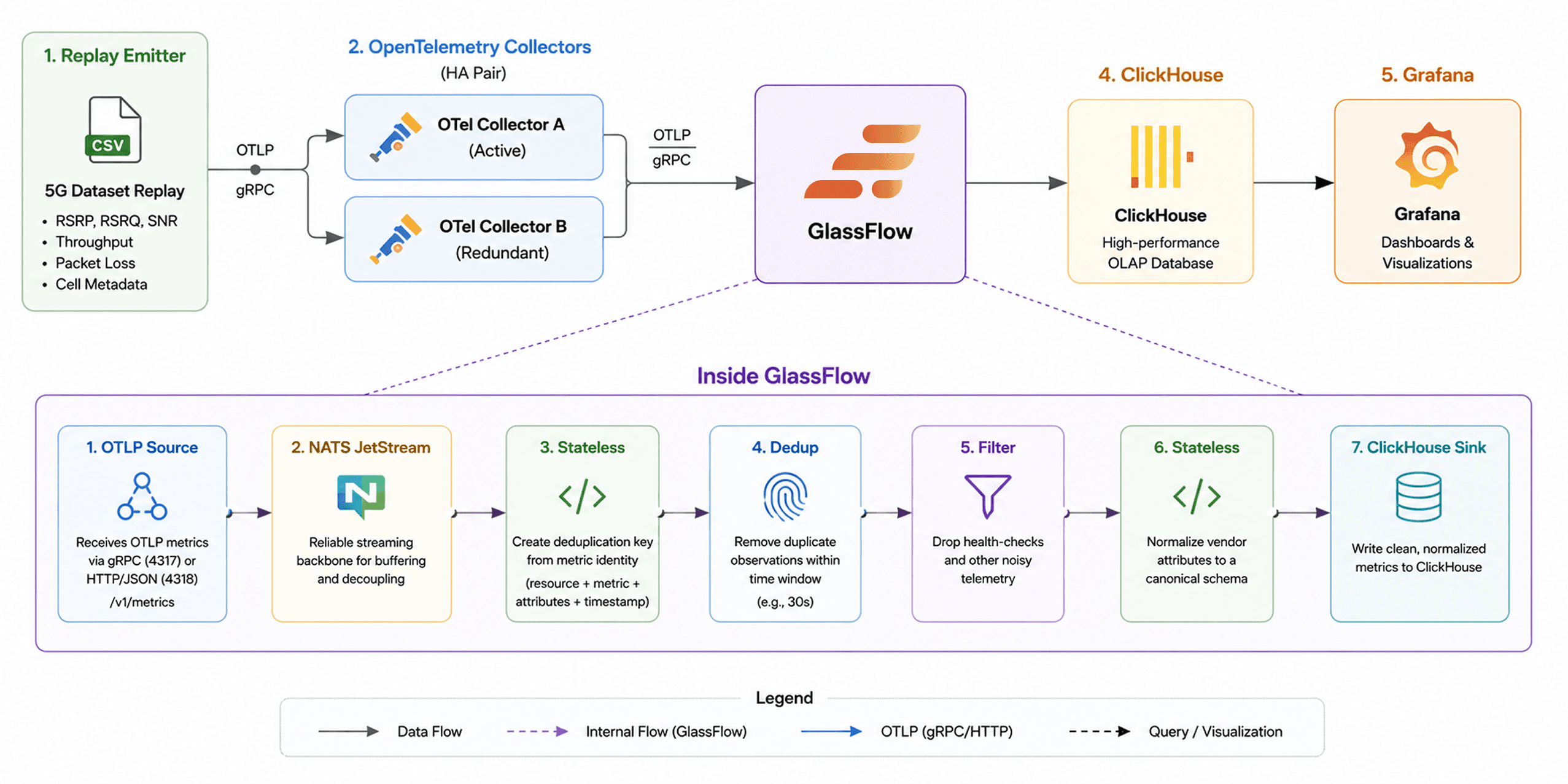
Figure 2. End-to-end OpenTelemetry pipeline for processing 5G signal-quality metrics. GlassFlow sits between OpenTelemetry and ClickHouse, applying deduplication, filtering, and schema normalization before the data reaches storage.

Processing the stream before it reaches ClickHouse allows us to store clean telemetry from the start. Unlike relying on ClickHouse's ReplacingMergeTree engine to clean duplicates post-ingestion, GlassFlow removes them upstream, reducing write amplification and simplifying ClickHouse table design. As metrics flow through GlassFlow, duplicate observations are removed, irrelevant telemetry is filtered out, and vendor-specific attributes are normalized into a consistent schema.

By performing these operations in the streaming layer, we ensure that only high-quality, analysis-ready data is written to ClickHouse, reducing storage overhead and simplifying downstream queries.

The Dataset: Real 5G Traces, Real Signal Degradation

To make the demo realistic, we'll use the publicly available 5G dataset from the University College Cork Mobile and Internet Systems Laboratory (UCCMISL). The dataset contains real-world mobile network measurements collected using G-NetTrack Pro across Cork, Ireland and includes nearly 189,000 observations spanning 83 CSV files.

Dataset repository here:

What makes this dataset useful for observability demonstrations is that it captures real-world variations in mobile network quality, including changes in signal strength, throughput, and network conditions. The traces include both static and driving scenarios, allowing us to observe realistic degradation events, handovers, and transitions between 5G and LTE.

For this article, we'll replay the measurements as a live telemetry stream. Each row is converted into OpenTelemetry metrics and emitted through a pair of OpenTelemetry Collectors, creating realistic duplicate telemetry patterns. We also inject a small amount of synthetic noise and schema variation to show how GlassFlow performs deduplication and data cleaning before the data reaches ClickHouse.

Table 1: Dataset At a Glance

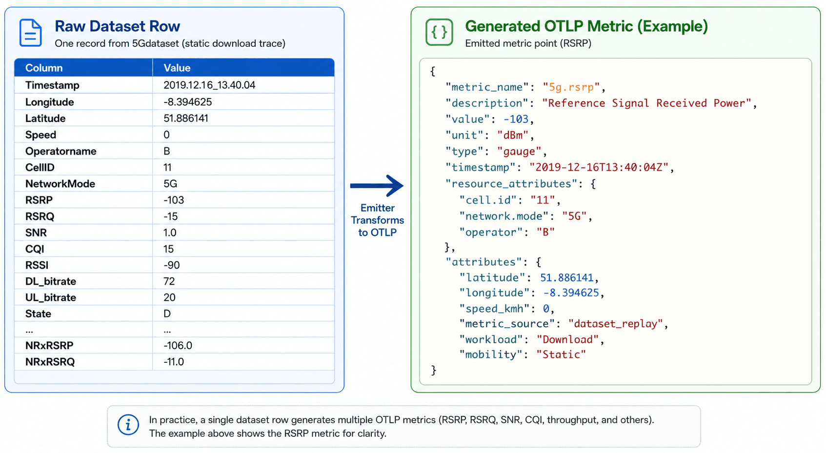
Figure 3. Converting a 5G dataset CSV record into an OpenTelemetry OTLP metric during replay

How Duplicate Telemetry Distorts 5G RAN Analytics

Our 5G telemetry stream flows through two OpenTelemetry Collectors configured for high availability. While this improves reliability, it also means the same metric can be exported twice.

For example, both collectors may observe and forward the same signal-quality measurement. Although both exports are valid, they represent a single observation and should only be counted once (Refer to Figure 1 for a visual explanation of this concept).

Hence, without deduplication, these duplicates can skew aggregations and add noise to dashboards. To address this, we'll use GlassFlow to remove duplicate observations before they reach ClickHouse. Because collectors may export data at slightly different times due to batching, retries, or network delays, we'll use a 30-second deduplication window to catch delayed duplicates.

In the next section, we'll build the GlassFlow pipeline that performs this deduplication and prepares the data for storage.

Deploying the Demo: Kubernetes + Helm Setup

To demonstrate the complete workflow, we'll deploy a local environment containing GlassFlow, ClickHouse, Grafana, two OpenTelemetry Collectors, and a telemetry emitter that replays the 5G dataset as live OTLP metrics.

All components run inside a local Kubernetes cluster and can be deployed with a few commands from the demo directory:

cd

cd

cd

Prerequisites

Before starting, make sure the following tools are installed:

• Docker

• Kind

• kubectl

• Helm

The 5G dataset is downloaded automatically by the replay emitter, so no manual dataset preparation is required.

Deploy the Environment

Create the local Kubernetes cluster and install the required components:

make cluster
make repos
make

make cluster
make repos
make

make cluster
make repos
make

Next, create the ClickHouse tables used by the demo:

make

make

make

Finally, deploy the GlassFlow pipeline:

# In a separate terminal
make pf-glassflow-api
# Main terminal
make

# In a separate terminal
make pf-glassflow-api
# Main terminal
make

# In a separate terminal
make pf-glassflow-api
# Main terminal
make

At this point, the entire environment is ready. The OpenTelemetry Collectors are configured to forward telemetry into GlassFlow, ClickHouse is ready to receive cleaned metrics, and Grafana is available for visualization.

Now let's examine the GlassFlow pipeline responsible for filtering, deduplicating, and normalizing the telemetry stream before it reaches storage.

The GlassFlow Pipeline, End to End

With the infrastructure in place, let's build the pipeline that processes the telemetry stream before it reaches ClickHouse.

The replay emitter sends every observation through two OpenTelemetry Collectors configured as a high-availability pair. Each collector exports the same signal-quality metrics to GlassFlow using OTLP. This creates the duplicate-emission pattern we discussed in the previous section and gives us a realistic stream to process.

The OTLP Source

Both collectors export directly to GlassFlow's OTLP endpoint. Because OTLP metrics have a predefined schema, GlassFlow automatically exposes fields such as metric names, timestamps, resource attributes, metric attributes, and values to downstream transformations.

Metrics flow directly from OpenTelemetry into GlassFlow using standard OTLP endpoints.

exporters:
  otlp:
    endpoint: glassflow-glassflow:4317
    headers:
      x-glassflow-pipeline-id: ran-5g-telemetry

service:
  pipelines:
    metrics:
      exporters

exporters:
  otlp:
    endpoint: glassflow-glassflow:4317
    headers:
      x-glassflow-pipeline-id: ran-5g-telemetry

service:
  pipelines:
    metrics:
      exporters

exporters:
  otlp:
    endpoint: glassflow-glassflow:4317
    headers:
      x-glassflow-pipeline-id: ran-5g-telemetry

service:
  pipelines:
    metrics:
      exporters

6.2. Filter: Remove Health-Check Noise

The replay process injects synthetic health-check metrics alongside the real signal-quality telemetry. These metrics are useful for validating pipeline health but add no value to downstream analytics.

The first stage removes these records before they consume storage or processing resources.

{
  "type": "filter",
  "source_id": "ran_metrics",
  "config": {
    "expression": "metric_name != 'ran.healthcheck'"
  }
}

{
  "type": "filter",
  "source_id": "ran_metrics",
  "config": {
    "expression": "metric_name != 'ran.healthcheck'"
  }
}

{
  "type": "filter",
  "source_id": "ran_metrics",
  "config": {
    "expression": "metric_name != 'ran.healthcheck'"
  }
}

6.3. Deduplication: Remove Duplicate Observations

Each replayed observation carries a unique measurement_id attribute. Since both collectors forward the same observation, the resulting metrics share the same identifier even though they arrive through different collection paths.

GlassFlow uses this identifier to remove duplicate observations within a 30-second window, ensuring that each measurement is written only once.

{
  "type": "dedup",
  "source_id": "ran_metrics",
  "config": {
    "key": "attributes.measurement_id",
    "time_window": "30s"
  }
}

{
  "type": "dedup",
  "source_id": "ran_metrics",
  "config": {
    "key": "attributes.measurement_id",
    "time_window": "30s"
  }
}

{
  "type": "dedup",
  "source_id": "ran_metrics",
  "config": {
    "key": "attributes.measurement_id",
    "time_window": "30s"
  }
}

6.4. Stateless Transformation: Normalize Vendor Attributes

To simulate a multi-vendor environment, the two collectors intentionally emit different attribute names for the same cell identifier.

For example:

A stateless transformation reconciles these variations into a single canonical field that downstream systems can query consistently.

{
  "type": "stateless",
  "source_id": "ran_metrics",
  "config": {
    "transforms": [
      {
        "expression": "resource_attributes['cell.id'] ?? resource_attributes['ran.cell.id'] ?? resource_attributes['network.element.id']",
        "output_name": "canonical_cell_id",
        "output_type": "string"
      }
    ]
  }
}

{
  "type": "stateless",
  "source_id": "ran_metrics",
  "config": {
    "transforms": [
      {
        "expression": "resource_attributes['cell.id'] ?? resource_attributes['ran.cell.id'] ?? resource_attributes['network.element.id']",
        "output_name": "canonical_cell_id",
        "output_type": "string"
      }
    ]
  }
}

{
  "type": "stateless",
  "source_id": "ran_metrics",
  "config": {
    "transforms": [
      {
        "expression": "resource_attributes['cell.id'] ?? resource_attributes['ran.cell.id'] ?? resource_attributes['network.element.id']",
        "output_name": "canonical_cell_id",
        "output_type": "string"
      }
    ]
  }
}

In addition to standardizing cell identifiers, the pipeline extracts commonly queried fields such as network mode, geographic coordinates, timestamps, and metric values into strongly typed columns that can be mapped directly into ClickHouse.

6.5. ClickHouse Sink

After filtering, deduplication, and normalization, the cleaned telemetry stream is written into ClickHouse.

The GlassFlow ClickHouse sink maps OpenTelemetry fields into typed ClickHouse columns while preserving the original attributes for ad-hoc analysis. This allows us to run efficient analytical queries without sacrificing access to the underlying telemetry context.

{
  "type": "clickhouse",
  "table": "ran_metrics",
  "max_batch_size": 1000,
  "max_delay_time": "1s",
  "mapping": [
    {
      "name": "canonical_cell_id",
      "column_name": "CellID"
    },
    {
      "name": "metric_name",
      "column_name": "MetricName"
    },
    {
      "name": "value_double",
      "column_name": "Value"
    },
    {
      "name": "timestamp",
      "column_name": "TimeUnix"
    }
  ]
}

{
  "type": "clickhouse",
  "table": "ran_metrics",
  "max_batch_size": 1000,
  "max_delay_time": "1s",
  "mapping": [
    {
      "name": "canonical_cell_id",
      "column_name": "CellID"
    },
    {
      "name": "metric_name",
      "column_name": "MetricName"
    },
    {
      "name": "value_double",
      "column_name": "Value"
    },
    {
      "name": "timestamp",
      "column_name": "TimeUnix"
    }
  ]
}

{
  "type": "clickhouse",
  "table": "ran_metrics",
  "max_batch_size": 1000,
  "max_delay_time": "1s",
  "mapping": [
    {
      "name": "canonical_cell_id",
      "column_name": "CellID"
    },
    {
      "name": "metric_name",
      "column_name": "MetricName"
    },
    {
      "name": "value_double",
      "column_name": "Value"
    },
    {
      "name": "timestamp",
      "column_name": "TimeUnix"
    }
  ]
}

6.6. The Complete Pipeline

The complete processing flow consists of four transformations applied to every incoming metric:

The full pipeline definition used in this demo is available in the repository:

At this point, the environment is ready. The OpenTelemetry Collectors are forwarding telemetry into GlassFlow, ClickHouse is prepared to store the processed metrics, and Grafana is available for visualization. The next step is to examine how GlassFlow transforms the incoming stream—filtering noise, removing duplicate observations, and normalizing attributes before the data reaches storage.

The ClickHouse Side: Queries, Validation, and Results

With the pipeline deployed and telemetry flowing, it's time to validate that the data arriving in ClickHouse is clean and ready for analysis.

One of the advantages of performing deduplication upstream is that ClickHouse can use a simple MergeTree table rather than relying on engines such as ReplacingMergeTree to clean up duplicates after ingestion. The database receives already-processed telemetry, allowing queries to operate directly on the data rather than compensating for inconsistencies.

Now, let’s port forward the desired ClickHouse services:

make

make

make

Running this will port forward the client and the HTTP API services within Kubernetes. Now, you can open your browser and go to http://localhost:8123 and click on the Web SQL UI to execute queries and get your results.

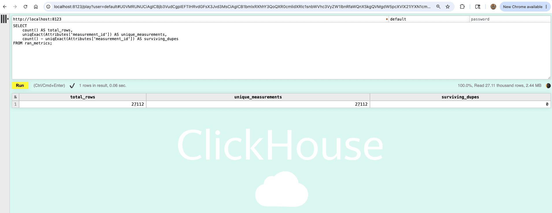
Figure 4. ClickHouse Web SQL UI showing RAN metrics query results at localhost:8123

Verify Deduplication

The first validation step is confirming that duplicate observations have been removed successfully.

Run the following query:

SELECT
    count() AS total_rows,
    uniqExact(Attributes['measurement_id']) AS unique_measurements,
    count() - uniqExact(Attributes['measurement_id']) AS surviving_dupes
FROM

SELECT
    count() AS total_rows,
    uniqExact(Attributes['measurement_id']) AS unique_measurements,
    count() - uniqExact(Attributes['measurement_id']) AS surviving_dupes
FROM

SELECT
    count() AS total_rows,
    uniqExact(Attributes['measurement_id']) AS unique_measurements,
    count() - uniqExact(Attributes['measurement_id']) AS surviving_dupes
FROM

If the pipeline is functioning correctly, surviving_dupes should be zero or very close to zero, confirming that duplicate observations emitted by the redundant collectors were removed before storage. You should see an output similar to this on your ClickHouse execution output:

Query id: 2eb122ef-2ff7-41f0-a55b-f41307246024

   ┌─total_rows─┬─unique_measurements─┬─surviving_dupes─┐
1. │      14219 │               14219 │               0

Query id: 2eb122ef-2ff7-41f0-a55b-f41307246024

   ┌─total_rows─┬─unique_measurements─┬─surviving_dupes─┐
1. │      14219 │               14219 │               0

Query id: 2eb122ef-2ff7-41f0-a55b-f41307246024

   ┌─total_rows─┬─unique_measurements─┬─surviving_dupes─┐
1. │      14219 │               14219 │               0

Detect Signal Degradation

One of the primary goals of the pipeline is to identify cells experiencing poor radio conditions.

The following query calculates a rolling average RSRP value for each cell:

Cells appearing in this result set are experiencing very weak signal conditions and may be candidates for further investigation. For the purposes of this demo, we just took a subset of the full dataset, so it will return only a few matching results. You should see an output similar to this:

Query id: 74324bee-e7a5-40d9-ac38-3319397423ad

    ┌──────────────minute─┬─CellID─┬────────────avg_rsrp─┐
 1. │ 2019-12-16 12:33:00 │ 3      │                -111 │
 2. │ 2019-12-16 12:33:00 │ 41     │                -114 │
 3. │ 2019-12-14 10:27:00 │ 3      │ -110.14285714285714 │
 4. │ 2019-12-14 10:26:00 │ 3      │ -111.06451612903226 │
 5. │ 2019-12-14 10:25:00 │ 3      │                -200 │
 6. │ 2019-11-29 10:17:00 │ 12     │ -113.81818181818181 │
 7. │ 2019-11-29 09:57:00 │ 1      │ -112.63636363636364 │
 8. │ 2019-11-29 09:56:00 │ 1      │ -111.79069767441861 │
 9. │ 2019-11-29 09:55:00 │ 1      │                -111 │
10. │ 2019-11-29 09:46:00 │ 1      │                -112

Query id: 74324bee-e7a5-40d9-ac38-3319397423ad

    ┌──────────────minute─┬─CellID─┬────────────avg_rsrp─┐
 1. │ 2019-12-16 12:33:00 │ 3      │                -111 │
 2. │ 2019-12-16 12:33:00 │ 41     │                -114 │
 3. │ 2019-12-14 10:27:00 │ 3      │ -110.14285714285714 │
 4. │ 2019-12-14 10:26:00 │ 3      │ -111.06451612903226 │
 5. │ 2019-12-14 10:25:00 │ 3      │                -200 │
 6. │ 2019-11-29 10:17:00 │ 12     │ -113.81818181818181 │
 7. │ 2019-11-29 09:57:00 │ 1      │ -112.63636363636364 │
 8. │ 2019-11-29 09:56:00 │ 1      │ -111.79069767441861 │
 9. │ 2019-11-29 09:55:00 │ 1      │                -111 │
10. │ 2019-11-29 09:46:00 │ 1      │                -112

Query id: 74324bee-e7a5-40d9-ac38-3319397423ad

    ┌──────────────minute─┬─CellID─┬────────────avg_rsrp─┐
 1. │ 2019-12-16 12:33:00 │ 3      │                -111 │
 2. │ 2019-12-16 12:33:00 │ 41     │                -114 │
 3. │ 2019-12-14 10:27:00 │ 3      │ -110.14285714285714 │
 4. │ 2019-12-14 10:26:00 │ 3      │ -111.06451612903226 │
 5. │ 2019-12-14 10:25:00 │ 3      │                -200 │
 6. │ 2019-11-29 10:17:00 │ 12     │ -113.81818181818181 │
 7. │ 2019-11-29 09:57:00 │ 1      │ -112.63636363636364 │
 8. │ 2019-11-29 09:56:00 │ 1      │ -111.79069767441861 │
 9. │ 2019-11-29 09:55:00 │ 1      │                -111 │
10. │ 2019-11-29 09:46:00 │ 1      │                -112

Throughput SLA Validation

Signal strength alone doesn't tell the whole story. Operators also care about the user experience delivered by the network.

The following query calculates the 95th percentile downlink throughput for each cell:

SELECT
    CellID,
    quantile(0.95)(Value) AS p95_throughput
FROM ran_metrics
WHERE MetricName = 'ran.dl_bitrate'
GROUP BY CellID
ORDER BY p95_throughput DESC

SELECT
    CellID,
    quantile(0.95)(Value) AS p95_throughput
FROM ran_metrics
WHERE MetricName = 'ran.dl_bitrate'
GROUP BY CellID
ORDER BY p95_throughput DESC

SELECT
    CellID,
    quantile(0.95)(Value) AS p95_throughput
FROM ran_metrics
WHERE MetricName = 'ran.dl_bitrate'
GROUP BY CellID
ORDER BY p95_throughput DESC

This type of query is commonly used for capacity planning, SLA reporting, and identifying underperforming cells. The demo will return the following output (numbers may vary a bit due to the randomness of the emitter):

Query id: 549a5b0d-f536-4fdc-af73-0a4f9a7ec353

    ┌─CellID─┬─────p95_throughput─┐
 1. │ 11     │ 156207.79999999996 │
 2. │ 12     │  50498.99999999996 │
 3. │ 13     │           22450.25 │
 4. │ 2      │              13869 │
 5. │ 41001  │ 11309.499999999998 │
 6. │ 52106  │            8713.25 │
 7. │ 3      │  6615.449999999997 │
 8. │ 20504  │               4286 │
 9. │ 40504  │ 3533.5999999999876 │
10. │ 8643   │ 3188.8999999999996 │
11. │ 10692  │             2733.7 │
12. │ 40506  │            1580.25 │
13. │ 30504  │             1562.5 │
14. │ 1      │ 1403.8999999999996 │
15. │ 57034  │              398.6 │
16. │ 52103  │ 340.79999999999995 │
17. │ 57031  │              136.7 │
18. │ 57185  │              37.75 │
19. │ 52089  │  15.59999999999999 │
20. │ 52083  │  4.249999999999998 │
21. │ 57099  │                  1 │
22. │ 52086  │                  0 │
23. │ 56991  │                  0 │
24. │ 10504  │                  0 │
25. │ 41     │                  0

Query id: 549a5b0d-f536-4fdc-af73-0a4f9a7ec353

    ┌─CellID─┬─────p95_throughput─┐
 1. │ 11     │ 156207.79999999996 │
 2. │ 12     │  50498.99999999996 │
 3. │ 13     │           22450.25 │
 4. │ 2      │              13869 │
 5. │ 41001  │ 11309.499999999998 │
 6. │ 52106  │            8713.25 │
 7. │ 3      │  6615.449999999997 │
 8. │ 20504  │               4286 │
 9. │ 40504  │ 3533.5999999999876 │
10. │ 8643   │ 3188.8999999999996 │
11. │ 10692  │             2733.7 │
12. │ 40506  │            1580.25 │
13. │ 30504  │             1562.5 │
14. │ 1      │ 1403.8999999999996 │
15. │ 57034  │              398.6 │
16. │ 52103  │ 340.79999999999995 │
17. │ 57031  │              136.7 │
18. │ 57185  │              37.75 │
19. │ 52089  │  15.59999999999999 │
20. │ 52083  │  4.249999999999998 │
21. │ 57099  │                  1 │
22. │ 52086  │                  0 │
23. │ 56991  │                  0 │
24. │ 10504  │                  0 │
25. │ 41     │                  0

Query id: 549a5b0d-f536-4fdc-af73-0a4f9a7ec353

    ┌─CellID─┬─────p95_throughput─┐
 1. │ 11     │ 156207.79999999996 │
 2. │ 12     │  50498.99999999996 │
 3. │ 13     │           22450.25 │
 4. │ 2      │              13869 │
 5. │ 41001  │ 11309.499999999998 │
 6. │ 52106  │            8713.25 │
 7. │ 3      │  6615.449999999997 │
 8. │ 20504  │               4286 │
 9. │ 40504  │ 3533.5999999999876 │
10. │ 8643   │ 3188.8999999999996 │
11. │ 10692  │             2733.7 │
12. │ 40506  │            1580.25 │
13. │ 30504  │             1562.5 │
14. │ 1      │ 1403.8999999999996 │
15. │ 57034  │              398.6 │
16. │ 52103  │ 340.79999999999995 │
17. │ 57031  │              136.7 │
18. │ 57185  │              37.75 │
19. │ 52089  │  15.59999999999999 │
20. │ 52083  │  4.249999999999998 │
21. │ 57099  │                  1 │
22. │ 52086  │                  0 │
23. │ 56991  │                  0 │
24. │ 10504  │                  0 │
25. │ 41     │                  0

Measuring the Impact of Deduplication (Optional)

To demonstrate why deduplication matters, the demo includes a second pipeline that intentionally preserves duplicate observations.

Deploy the no-dedup pipeline:

make deploy-pipeline-no-dedup
make switch-collectors-no-dedup
make

make deploy-pipeline-no-dedup
make switch-collectors-no-dedup
make

make deploy-pipeline-no-dedup
make switch-collectors-no-dedup
make

Then compare row counts against unique measurements:

SELECT
    CellID,
    count() AS rows,
    uniqExact(Attributes['measurement_id']) AS unique_measurements,
    count() / greatest(uniqExact(Attributes['measurement_id']), 1) AS inflation_factor
FROM ran_metrics
WHERE MetricName = 'ran.rsrp'
GROUP BY CellID
ORDER BY inflation_factor DESC
LIMIT 6

SELECT
    CellID,
    count() AS rows,
    uniqExact(Attributes['measurement_id']) AS unique_measurements,
    count() / greatest(uniqExact(Attributes['measurement_id']), 1) AS inflation_factor
FROM ran_metrics
WHERE MetricName = 'ran.rsrp'
GROUP BY CellID
ORDER BY inflation_factor DESC
LIMIT 6

SELECT
    CellID,
    count() AS rows,
    uniqExact(Attributes['measurement_id']) AS unique_measurements,
    count() / greatest(uniqExact(Attributes['measurement_id']), 1) AS inflation_factor
FROM ran_metrics
WHERE MetricName = 'ran.rsrp'
GROUP BY CellID
ORDER BY inflation_factor DESC
LIMIT 6

With deduplication disabled, the inflation factor approaches 2.0 because both collectors write the same observation. Once the deduplicated pipeline is restored, the inflation factor returns to 1.0.

This comparison illustrates the core value of the pipeline: analytics are only as trustworthy as the telemetry feeding them

Visualizing the Results in Grafana

The demo includes a pre-configured Grafana dashboard connected directly to ClickHouse.

Launch Grafana:

make

make

make

Then open http://localhost:3000 and log in using admin/admin. You will be asked to set a new password on first login so please do so. Then, you can navigate to the Dashboards section where you should see the preconfigured dashboard.

The dashboard provides a real-time view of the processed telemetry stream, including:

• Per-cell RSRP trends

• Throughput heatmaps

• SLA breach indicators

• Deduplication comparison panels

As the replay progresses, signal degradation events from the dataset become visible in near real time. Because GlassFlow has already filtered noise, removed duplicate observations, and normalized attributes, the dashboard reflects actual network conditions rather than artifacts introduced by the telemetry pipeline.

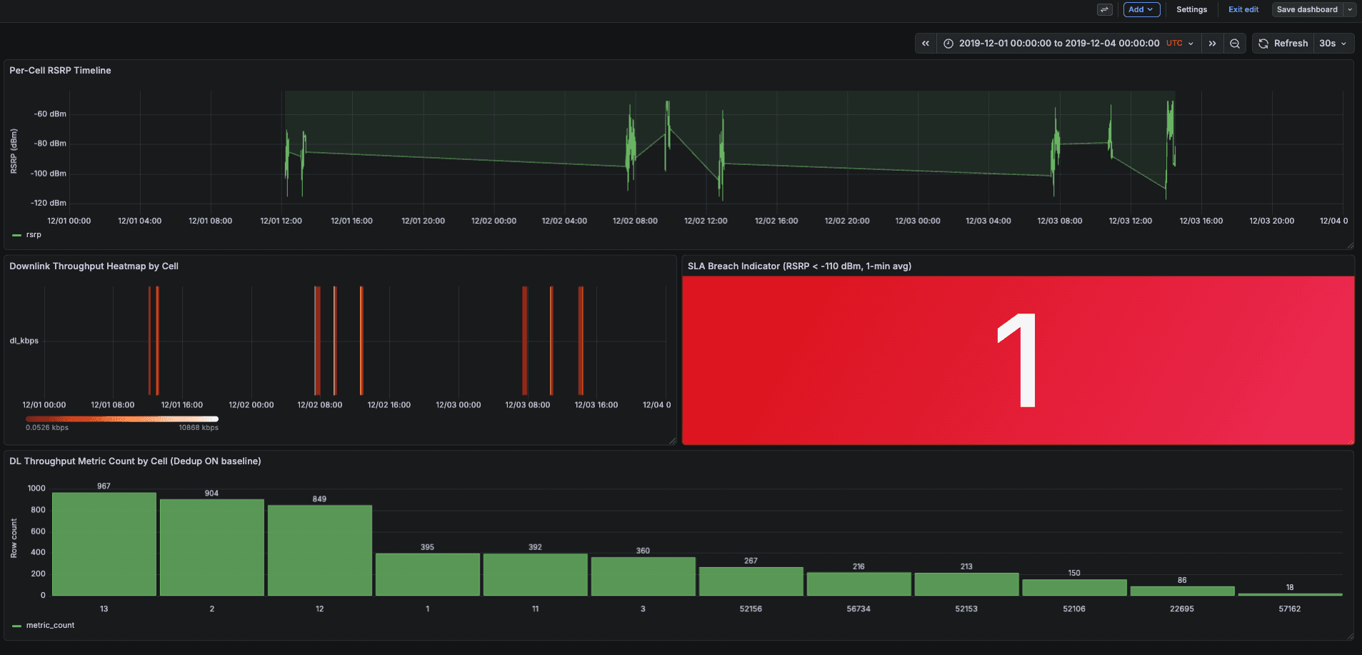
Figure 5. Grafana dashboard showing per-cell RSRP signal quality trends, throughput heatmaps, and deduplication comparison panels

Results: What Upstream Deduplication Achieves

This demo demonstrates three things:

• Duplicate observations emitted by redundant OpenTelemetry Collectors can be removed before they reach the analytics layer.

• Vendor-specific attribute naming can be normalized into a consistent schema during stream processing.

• An OTLP-native architecture is sufficient for real-time telemetry processing, eliminating the need for additional messaging infrastructure in this workflow.

It also demonstrates the operational value of upstream processing. By the time telemetry reaches ClickHouse, it is already filtered, deduplicated, and normalized, allowing dashboards and analytical queries to operate on clean data.

At the same time, this is not the only valid approach. ClickHouse features such as ReplacingMergeTree can also be used to address duplicate records in some workloads. This article focuses on upstream stream processing as an alternative that is particularly well-suited to high-volume telemetry pipelines.

Finally, while the telemetry traces come from a real-world 5G dataset, the dual-collector deployment is intentionally simulated. The goal is to reproduce the duplicate-emission patterns commonly seen in production high-availability collector topologies.

Production Considerations for RAN Telemetry Pipelines

A few practical considerations are worth keeping in mind when adapting this pattern to production environments:

• Choose a deduplication window that comfortably covers collector batching, retries, and network latency.

• Apply deduplication selectively. It provides the most value for high-volume telemetry streams where duplicate observations can significantly impact analytics.

• Normalize attributes as early as possible to avoid carrying vendor-specific complexity into dashboards and queries.

• Treat stream processing and analytics as separate concerns: GlassFlow prepares the data, while ClickHouse focuses on storing and querying it efficiently.

Conclusion: Clean Telemetry Starts at the Source

5G observability pipelines generate large volumes of telemetry, but volume alone does not create useful insights. Duplicate observations, inconsistent schemas, and operational noise can all reduce the accuracy of downstream analytics.

In this tutorial, we used GlassFlow to process OpenTelemetry metrics before they reached ClickHouse. A simple pipeline—filtering health checks, removing duplicate observations, and normalizing attributes—turned a noisy telemetry stream into a trustworthy one.

The broader lesson extends beyond telecommunications: cleaning data before it reaches the database is often simpler and more efficient than compensating for data quality issues afterward.

If you'd like to try it yourself, clone the demo repository, replay the dataset, and compare the results with deduplication enabled and disabled. The difference becomes apparent almost immediately.

Want to run GlassFlow in your own pipeline? Get started here.

References

• GlassFlow OTLP Source Documentation

• GlassFlow Deduplication Transformation

• GlassFlow Stateless Transformation

• GlassFlow Pipeline Configuration Reference (v3)

• GlassFlow ClickHouse Sink

• GlassFlow Data Flow Architecture

• GlassFlow ClickHouse ETL Repository

• uccmisl/5Gdataset

• OpenTelemetry Metrics Data Model Specification

• Solving the "Latest State" Problem in ClickHouse with Real-Time Deduplication

Frequently Asked Questions

What is OpenTelemetry (OTel)?
OpenTelemetry is an open-source observability framework that standardizes how telemetry data (metrics, logs, traces) is collected, instrumented, and exported. It's vendor-neutral and supported by all major cloud providers and observability vendors.

What causes duplicate metrics in OpenTelemetry pipelines?
Duplicate metrics occur when redundant OpenTelemetry Collectors, deployed for high availability, each forward the same observation to the downstream backend. Without deduplication, a single measurement appears twice in storage, inflating counts and skewing aggregations.

Why use GlassFlow instead of deduplicating in ClickHouse?
Deduplicating in ClickHouse (via ReplacingMergeTree) requires extra storage for duplicate rows before merges run, complicates query logic, and adds operational overhead. GlassFlow removes duplicates in the streaming layer before any data reaches ClickHouse, keeping the database simple and queries accurate from the start.

What is RAN signal quality degradation?
RAN (Radio Access Network) signal quality degradation refers to a deterioration in the radio signal between a 5G base station (gNB) and a user device. It's measured via metrics such as RSRP (Reference Signal Received Power), RSRQ (Reference Signal Received Quality), and SNR (Signal-to-Noise Ratio). Degradation can indicate interference, coverage gaps, or hardware issues.

What is OTLP?
OTLP (OpenTelemetry Protocol) is the native wire protocol used to transmit telemetry data between OpenTelemetry Collectors and backends. GlassFlow accepts OTLP natively, meaning no additional message queue (Kafka, Pulsar) is needed to connect OTel to GlassFlow.

Can this pipeline work in production with real 5G infrastructure?
Yes. The architecture dual OTel Collectors → GlassFlow → ClickHouse mirrors production high-availability collector topologies. The main adjustments for production are sizing the deduplication window to match your collector batching intervals and tuning ClickHouse batch sizes.