ljn
ClickHouse Learnings
Learn ClickHouse JOINs step by step: types, examples & best practices.
Written by
Armend Avdijaj
-

Mastering JOINs in ClickHouse
TL;DR: Key Takeaways
Denormalize First, Join Second: ClickHouse is built for speed on wide, denormalized tables. Use JOINs strategically for flexibility, not as the default.
Use the Right
JOINfor the Job: Go beyondINNERandLEFT. UseANY JOINfor fast lookups,ASOF JOINfor time-series data, andSEMI/ANTI JOINfor efficient filtering.Performance is in Your Hands: Always put the smaller table on the right side of the
JOIN. Filter data as early as possible in your query to reduce the amount of data being processed.Know the Algorithms: ClickHouse uses different algorithms like
Hash Join(fast, memory-intensive) andMerge Join(good for sorted data). Understanding these helps you tune for speed or low memory usage.Mind the Limitations: Be aware that JOINs can be memory-heavy. For distributed queries across a cluster, use
GLOBAL JOINto ensure correctness.
Why JOINs in a Columnar World?
ClickHouse is an open-source, column-oriented database management system (DBMS) engineered for online analytical processing (OLAP). Its architecture is built for speed, capable of processing billions of rows and terabytes of data to generate analytical reports in milliseconds. This performance stems from its columnar storage model. Unlike traditional row-based databases that store all values for a single row together, ClickHouse stores all values for a single column together. This design is revolutionary for analytical queries because it enables the database to read only the specific columns required for a query, thereby drastically reducing disk I/O and accelerating aggregations such as SUM, AVG, and COUNT.
To achieve this lightning-fast performance, the recommended data modeling practice in ClickHouse is denormalization. This approach involves creating large, wide, "flat" tables that contain all the information needed for analysis in a single place. By pre-joining data during the ingestion or ETL (Extract, Transform, Load) process, denormalization eliminates the need for expensive JOIN operations at query time, leading to simpler and faster query execution.
However, pure denormalization is not always practical. It can lead to significant data redundancy, increased storage costs, and complex data update logic, as a single piece of information might need to be changed in many rows. In contrast, a normalized schema, which separates data into distinct logical tables (e.g., orders, customers, products), offers greater flexibility, easier data management, and reduced redundancy. This is where JOINs become essential.
Contrary to some misconceptions, JOINs are fully supported in ClickHouse, which offers a rich toolkit of standard and specialized JOIN types. However, consider them a powerful feature to use strategically, rather than a default data modeling tool. The extensive development of multiple JOIN types and sophisticated execution algorithms within ClickHouse is a clear acknowledgment that real-world applications often demand the flexibility that JOINs provide, especially for ad-hoc exploratory analysis or when denormalization is prohibitively complex. This guide will navigate the landscape of ClickHouse JOINs, teaching how to use this powerful capability effectively by understanding its unique characteristics, performance implications, and underlying mechanics.
A Refresher on Standard SQL JOINs
Before diving into the specifics of ClickHouse, it is crucial to have a solid foundation in standard SQL JOINs. A JOIN clause is used to combine rows from two or more tables based on a related column between them, known as a join key.
A popular way to visualize JOINs is with Venn diagrams, which represent tables as overlapping circles. While intuitive, this analogy has limitations that I will address shortly.
Also, I will be using the following two tables for the examples.
Product Table
Order Table
Inner Join
Inner join only returns the rows that have matching values in both tables.

Inner Join
Left Outer Join
Left outer join returns all rows from the left table (TableA), and the matched rows from the right table (TableB). If there is no match, the columns from the right table will contain default values (often NULL).

Left Outer Join
Right Outer Join
Right outer join returns all rows from the right table (TableB), and the matched rows from the left table (TableA). If there is no match, the columns from the left table will contain default values.
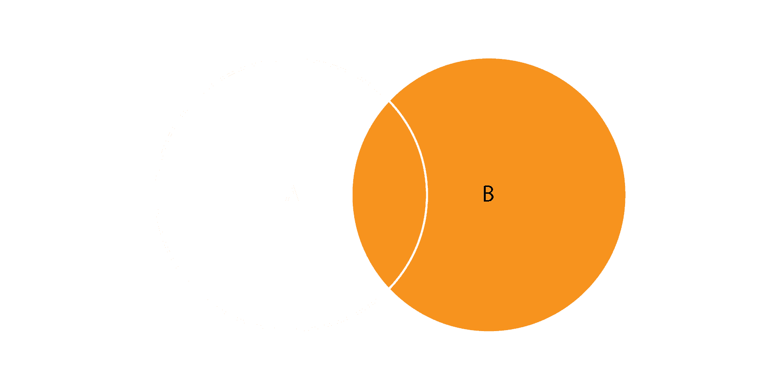
Right Outer Join
Full Outer Join
Full outer join returns all rows when there is a match in either the left or the right table. It combines the functionality of LEFT and RIGHT JOIN.
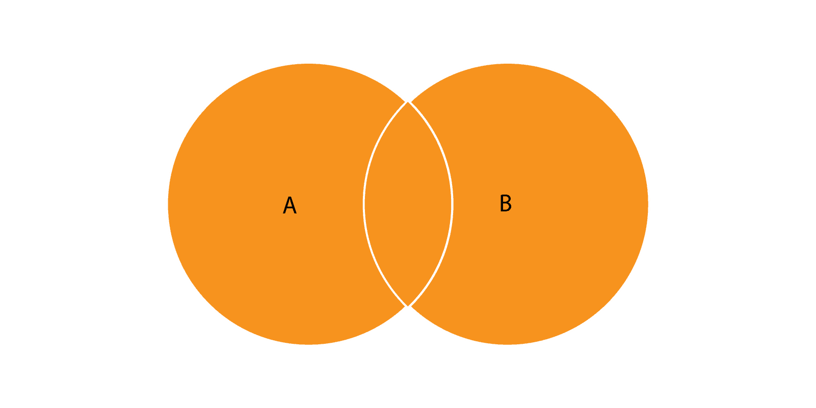
Full Outer Join
Why Venn Diagrams Can Be Misleading
While helpful for initial understanding, Venn diagrams are technically inaccurate for explaining SQL JOINs. Venn diagrams illustrate set operations like UNION, INTERSECT, and EXCEPT, which operate on sets of elements of the same type. A SQL JOIN is fundamentally different. It is not a set operation but a filtered Cartesian product.
Here is a more accurate mental model:
Cartesian Product (
CROSS JOIN): First, the database engine conceptually creates a massive intermediate table by pairing every single row from the left table with every single row from the right table. IfTable_Ahas 1,000 rows andTable_Bhas 1,000 rows, theCROSS JOINproduces 1,000,000 rows.Filtering (
ONclause): Next, the engine filters this huge intermediate table, keeping only the rows where the condition in theONclause is true (e.g.,Table_A.key = Table_B.key).
This model correctly explains why a JOIN can sometimes produce more rows than exist in either of the original tables. If a key in Table_A matches three keys in Table_B, the final result will include three rows for that single key from Table_A. A Venn diagram cannot represent this multiplicative behavior. Understanding this "Cartesian Product -> Filter" mechanism is the key to mastering JOINS, especially in a high-performance database like ClickHouse.
ClickHouse JOIN
ClickHouse supports all standard SQL JOIN types and enhances them with specialized modifiers and entirely new JOIN types designed for analytical workloads. These are not just syntactic sugar; they are purpose-built tools that can dramatically improve query performance and solve specific analytical problems.
Strictness Modifiers: ANY and ALL
In standard SQL, JOINs implicitly use ALL strictness. This means if a single row from the left table matches multiple rows in the right table, all possible combinations are returned, forming a Cartesian product for those matching keys. While this is sometimes necessary, it can lead to an explosion in result set size and is often inefficient for simple data enrichment.
ClickHouse introduces the ANY strictness modifier as a powerful optimization. An ANY JOIN returns only the first found matching row from the right table for each key from the left table, effectively disabling the Cartesian product.
This makes ANY JOIN exceptionally fast and memory-efficient for lookup scenarios. For example, if enriching an orders table with customer names from a customers table, an ANY JOIN is ideal because each order belongs to only one customer, and only one name needs to be attached.
Now, let's compare LEFT ALL JOIN (the default) with LEFT ANY JOIN.
Query with ALL strictness (implicit):
Result: Notice that Alice appears twice, once for each of her logins.
Query with ANY strictness:
For simple lookups, ANY JOIN is the clear winner in terms of performance and memory usage.
Filtering JOIN: SEMI and ANTI
Sometimes, the goal is not to combine columns but to filter one table based on the contents of another. ClickHouse provides two highly efficient JOIN types for this purpose: SEMI JOIN and ANTI JOIN.
SEMI JOIN: Returns rows from the left table for which a matching key exists in the right table. It does not add any columns from the right table and, likeANY JOIN, returns each left-side row only once, even if there are multiple matches on the right. This is often a more performant alternative to aWHERE... IN (SELECT...)subquery.ANTI JOIN: The logical opposite ofSEMI JOIN. It returns rows from the left table for which no matching key exists in the right table. This is an efficient way to perform aNOT EXISTSor aLEFT JOIN... WHERE right_table.key IS NULLoperation.
To illustrate this feature, let’s create products and sales tables.
LEFT SEMI JOIN: Find all products that have been sold
Result: Returns only the products that have an entry in the sales table.
LEFT ANTI JOIN: Find all products that have never been sold
Result: Returns the 'Mouse', which has no corresponding entry in the sales table.
Time-Series Magic: ASOF JOIN
The ASOF JOIN is a specialized tool designed for time-series analysis. It performs a non-exact match, joining rows from the left table with the row from the right table that has the closest preceding timestamp (or any other ordered numeric key).
Its syntax requires two types of conditions in the ON clause:
An exact match condition on one or more keys (e.g.,
ON trades.symbol = quotes.symbol).A closest match condition on an ordered key, typically a timestamp (e.g.,
AND trades.time >= quotes.time).
This is invaluable for scenarios like attaching a stock quote to a trade, where the quote's timestamp will almost never exactly match the trade's timestamp. ASOF JOIN finds the last valid quote before the trade occurred.
Let's create trades and quotes tables.
Now let’s find the price for each trade based on the most recent quote at the time of the trade.
Result:
The first trade at 10:00:05 is matched with the quote from 10:00:00. The second trade at 10:00:12 is matched with the quote from 10:00:10, which was the most recent quote before the trade.
A Special Case: Unnesting with ARRAY JOIN
While it uses the JOIN keyword, ARRAY JOIN is not a traditional join between two tables. Instead, it is a powerful operator that "unfolds" or "unnests" an array column, creating a new row for each element in the array while duplicating the values in all other columns.
This is extremely useful for analyzing data stored in arrays. For example, if a table of articles has a column tags Array(String), ARRAY JOIN can be used to create a row for each tag, allowing for aggregations like counting the usage of each tag. The LEFT ARRAY JOIN variant will produce a row even if the array is empty, which can be useful for preserving the original row count.
Let’s see it in action.
Now let’s unnest the tags to count how many articles are associated with each tag.
Result: The row for article 3 is excluded because its tags array is empty.
The Summary of ClickHouse JOIN Toolkit
The following table serves as a quick-reference guide to help select the appropriate JOIN type for various analytical tasks.
JOIN Type | Syntax Example | Core Function | Best Use Case |
|---|---|---|---|
ALL JOIN |
| Returns all matching rows (Cartesian product for duplicates). | When you need every combination of matching rows from both tables. |
ANY JOIN |
| Returns only the first found matching row from the right table. | Fast data enrichment or lookups where only one match is needed. |
SEMI JOIN |
| Filters the left table, keeping rows that have a match in the right table. | Efficiently checking for the existence of related data (e.g., "users with orders"). |
ANTI JOIN |
| Filters the left table, keeping rows that have no match in the right table. | Finding records that lack a relationship (e.g., "products without sales"). |
ASOF JOIN |
| Performs a non-exact match based on the closest preceding ordered key. | Time-series analysis, such as matching trades to quotes or events to states. |
ARRAY JOIN |
| Unnests an array column, creating a new row for each element. | Analyzing and aggregating data stored within arrays. |
A Peak Under the Hood at JOIN Algorithms
The performance of a JOIN in ClickHouse depends not only on its type (INNER, LEFT, etc.) but critically on the underlying algorithm used to execute it. ClickHouse features a number of join algorithm, each with distinct trade-offs between memory consumption and execution speed. While ClickHouse can often select an appropriate algorithm automatically (by setting join_algorithm = 'auto'), understanding these mechanisms empowers users to make informed tuning decisions for complex queries.
The Default Workhorse: Hash-Based Joins
Hash-based algorithms are the most common and versatile in ClickHouse. They operate by building an in-memory hash table (similar to a dictionary or map) of the right-hand table, which allows for very fast lookups.
Hash Join: This is the most generic algorithm and supports all
JOINtypes. It follows a two-phase process:Build Phase: The entire right-hand table is streamed into memory, and a hash table is constructed using the join key(s) as the hash keys.
Probe Phase: The left-hand table is streamed row by row and joined by doing lookups into the hash table.
Parallel Hash Join: This is an enhancement of the standard
Hash Join. The "Build Phase" is parallelized across multiple CPU cores, which significantly speeds up the creation of the hash table for larger right-side tables. However, this comes at the cost of higher peak memory consumption.Grace Hash Join: This is the solution for when the right-hand table is too large to fit into memory. It is a non-memory-bound algorithm that avoids failure by "spilling" data to temporary storage on disk. It partitions both tables into smaller buckets using a hash function and then performs a standard
Hash Joinon each pair of corresponding buckets that can fit in memory.
Leveraging Order: Merge-Based Join
Merge-based algorithms are designed to be highly efficient when data is sorted on the join key.
Full Sorting Merge Join: This algorithm first ensures both the left and right tables are sorted by the join key. It then merges the two sorted streams in a single, efficient pass, much like merging two sorted lists. Its most powerful feature is an optimization: if a table is already physically sorted on disk by its primary key (defined in the
ORDER BYclause of theCREATE TABLEstatement), the expensive sorting step for that table can be skipped entirely. This can make it extremely fast and memory-efficient.Partial Merge Join: This algorithm is optimized for scenarios with very low memory. It always fully sorts the right table to disk and creates on-disk indexes for it. It then reads the left table block by block, sorts each block in memory, and uses the indexes to efficiently join with the corresponding data from the right table on disk. It is generally slower but has the lowest memory footprint of the non-memory-bound algorithms.
The Ultimate Speed: Direct Join
The Direct Join is the fastest algorithm available but comes with specific prerequisites. It completely eliminates the "Build Phase" of a hash join.
How it Works: This algorithm can only be used when the right-hand table is a data structure that already supports fast key-value lookups, such as a ClickHouse Dictionary, a table using the
Joinengine, orEmbeddedRocksDB. Because the key-value map is already built and loaded in memory, theJOINbecomes a series of highly optimized direct lookups as the left table is streamed.Limitations: Its primary limitation is that it generally only supports
LEFT ANY JOINsemantics, as key-value structures like dictionaries typically enforce unique keys.
Choosing the Right JOIN Algorithm
The choice of algorithm is a direct negotiation with the physical constraints of the system, primarily RAM and disk I/O. The hierarchy from Direct Join down to Partial Merge Join represents a spectrum of trade-offs between performance and flexibility. The following table provides a practical guide for selecting an algorithm based on common scenarios.
Scenario | Recommended Algorithm | Key Consideration |
|---|---|---|
My right table is a small, frequently used key-value lookup table. | Direct Join | Requires pre-configuring the right table as a ClickHouse Dictionary. Offers the absolute best performance. |
My right table is small to medium-sized and fits comfortably in RAM. | Parallel Hash Join (default) | The fastest and most versatile general-purpose algorithm. |
Both tables are very large and already sorted on the join key. | Full Sorting Merge Join | Extremely memory-efficient and fast in this specific case, as it skips the sorting step. |
My right table is too large to fit in RAM. | Grace Hash Join | A flexible non-memory-bound option that spills to disk. Performance is tunable. |
I have extremely limited memory, and performance is a secondary concern. | Partial Merge Join | The slowest of the non-memory-bound options but uses the least amount of RAM. |
Performance Playbook: Optimizing Your ClickHouse JOINs
Unlike traditional databases with highly sophisticated, cost-based optimizers, ClickHouse JOIN performance benefits immensely from thoughtful query design and manual tuning. The core principle behind nearly every optimization is to reduce the amount of data processed at every stage of the query. The following practices are a playbook for writing efficient JOINs.
The Golden Rule: Smaller Table on the Right: For hash-based joins, ClickHouse builds an in-memory hash table from the right-hand side of the
JOIN. Therefore, always place the smaller of the two tables on the right. This minimizes the memory required for the hash table and reduces the time spent in the "Build Phase". While recent versions of ClickHouse (24.12+) have a query planner that can automatically reorder tables, understanding this principle is fundamental to writing performant JOINs.Avoid Cartesian Products with
ANY JOIN: As discussed earlier, if a join key in the left table matches multiple rows in the right table, a standard (ALL)JOINwill return all combinations. For data enrichment or lookup tasks where only a single match is needed, usingANY JOINis the single most effective optimization. It prevents the result set from exploding in size and is significantly faster and less memory-intensive.Filter Early and Often: Reduce the amount of data entering the
JOINoperation by applying filters in theWHEREclause as early as possible. ClickHouse's query planner attempts to "push down" predicates to the underlying tables before the join, but explicitly filtering both tables in subqueries or withWHEREconditions is a robust practice that guarantees less data is processed by the join algorithm.Inefficient (JOIN first, then filter)
Efficient (Filter first, then JOIN)
Use
INInstead ofJOINfor Existence Checks: When the goal is simply to filter one table based on the existence of keys in another (the use case forSEMI JOIN), using aWHERE... IN (subquery)clause is often much faster. TheINoperator only needs to build a hash set of the keys from the subquery and check for existence, avoiding the overhead of retrieving and combining columns from the right table.Optimize Join Key Data Types: The performance of a
JOINis sensitive to the data types of the join keys. Use the smallest integer types possible (e.g.,UInt32instead ofUInt64if the cardinality allows). AvoidNullabletypes for join keys unless absolutely necessary, as they introduce extra overhead for handlingNULLvalues.Leverage Sorting Keys for Merge Joins: If two large tables are frequently joined on the same set of columns, a powerful optimization is to include those columns in the
ORDER BYclause of bothCREATE TABLEstatements. This physically sorts the data on disk by those keys. When afull_sorting_mergejoin is later performed on these keys, ClickHouse can skip the expensive in-memory or external sorting step, resulting in a very fast and memory-efficient join.Understand Distributed Joins (
GLOBAL JOIN): In a distributed ClickHouse cluster, a standardJOINis executed locally on each shard. Each shard builds a right-hand table using only its local data. This is often not the desired behavior. To join a large, sharded table (on the left) with a smaller dimension table (on the right), useGLOBAL... JOIN. This syntax instructs the initiator node to first compute the entire right-hand table, broadcast this complete table to every shard, and then perform the join on each shard against the full dimension table.
Navigating the Limitations
No database is a universal solution, and ClickHouse's design choices, which make it exceptionally fast for its core use cases, also introduce certain limitations for JOINs. Understanding these limitations is key to avoiding common pitfalls and working effectively with the database's architecture. These are not arbitrary flaws but rather the logical consequences of a design optimized for speed on single-table analytical scans.
Rule-Based Query Planner: Historically, ClickHouse has used a rule-based query planner. Unlike a cost-based planner that analyzes data statistics to find the most efficient execution path, a rule-based planner follows a fixed set of heuristics. This can sometimes lead to suboptimal plans for complex queries with multiple JOINs, which is why manual tuning (like ordering tables and filtering early) is so crucial. It should be noted that ClickHouse is actively developing a more advanced, cost-based planner known as the "Analyzer" to mitigate this.
Memory Consumption and Guardrails: The default hash-based join algorithms are memory-intensive. If the right-hand table is too large to fit in the available RAM, the query will fail with an "out of memory" error by default. To prevent this, ClickHouse provides "guardrail" settings like
max_rows_in_joinandmax_bytes_in_join, which will cause the query to fail gracefully if aJOINoperation exceeds these thresholds. These settings prevent server instability but require the user to either provision more memory, filter the data more aggressively, or switch to a non-memory-bound algorithm likeGrace Hash JoinorPartial Merge Join.Distributed
JOINChallenges: ClickHouse's distributed execution model is designed for "shared-nothing" parallelism, where each node works independently on its local data to minimize network communication. This is highly efficient for aggregations but presents a challenge forJOINs. ClickHouse does not support "data shuffling," a process used by systems like Apache Spark where data is dynamically repartitioned and sent between nodes to co-locate matching join keys. The absence of shuffling is a trade-off for faster execution of single-table distributed queries. The workaround for many distributedJOINscenarios is theGLOBAL JOINsyntax, which involves a potentially large, one-time broadcast of the right table to all nodes.Restrictions on Join Keys: There are several specific restrictions on the types of conditions and data used in join keys:
Inequality Conditions: Conditions using operators like
>or<are only supported by thehashandgrace_hashjoin algorithms and are incompatible with thejoin_use_nullssetting.NULL Handling: By default,
NULLvalues in a join key do not match anything, including otherNULLvalues. This is standard SQL behavior but can be surprising to newcomers.Type Compatibility: ClickHouse can perform implicit type casting on join keys, but the
JOINwill fail if there is no common, compatible data type. For instance, aJOINbetween aStringand anInt32key is not possible.
To learn more see our previous article.
Conclusion
JOINs in ClickHouse are a deep and powerful feature, reflecting the database's evolution from a specialized analytics engine to a more comprehensive data warehouse. While ClickHouse's columnar architecture and performance philosophy will always favor denormalized, flat table structures, its robust support for JOINs provides the critical flexibility needed for modern, complex analytical applications.
Mastering JOINs in this environment requires a shift in mindset away from the patterns of traditional OLTP databases. Success hinges on a strategic approach that acknowledges the underlying mechanics of the system.
The key takeaways are:
Denormalize by Default, Join by Design: Start with denormalization as the primary strategy for high-performance, high-concurrency workloads. Use JOINs deliberately for data enrichment, ad-hoc analysis, or where the complexity of maintaining a denormalized view is too high.
Use the Right Tool for the Job: Go beyond standard JOINs. Leverage ClickHouse's specialized toolkit—use
ANY JOINfor fast lookups,ASOF JOINfor time-series analysis, andSEMI/ANTI JOINfor efficient filtering.Understand the Engine Room: The choice of
JOINalgorithm is a critical performance lever. Understand the trade-offs between the speed of in-memoryHashjoins and the resilience of disk-spillingGrace HashandMergejoins. Guide the planner when necessary.Optimize Aggressively: Performance is in the user's hands. Aggressively reduce the data being joined by filtering early, using the smallest possible key types, and always placing the smaller table on the right side of the
JOIN.
The ClickHouse team is continuously improving JOIN performance, with recent releases introducing a more intelligent query planner and faster algorithms. By combining these ongoing platform enhancements with the principles and techniques outlined in this guide, developers and analysts can confidently and effectively harness the full power of JOINs to build sophisticated, high-performance analytical systems on ClickHouse.
Did you like this article? Share it!
You might also like
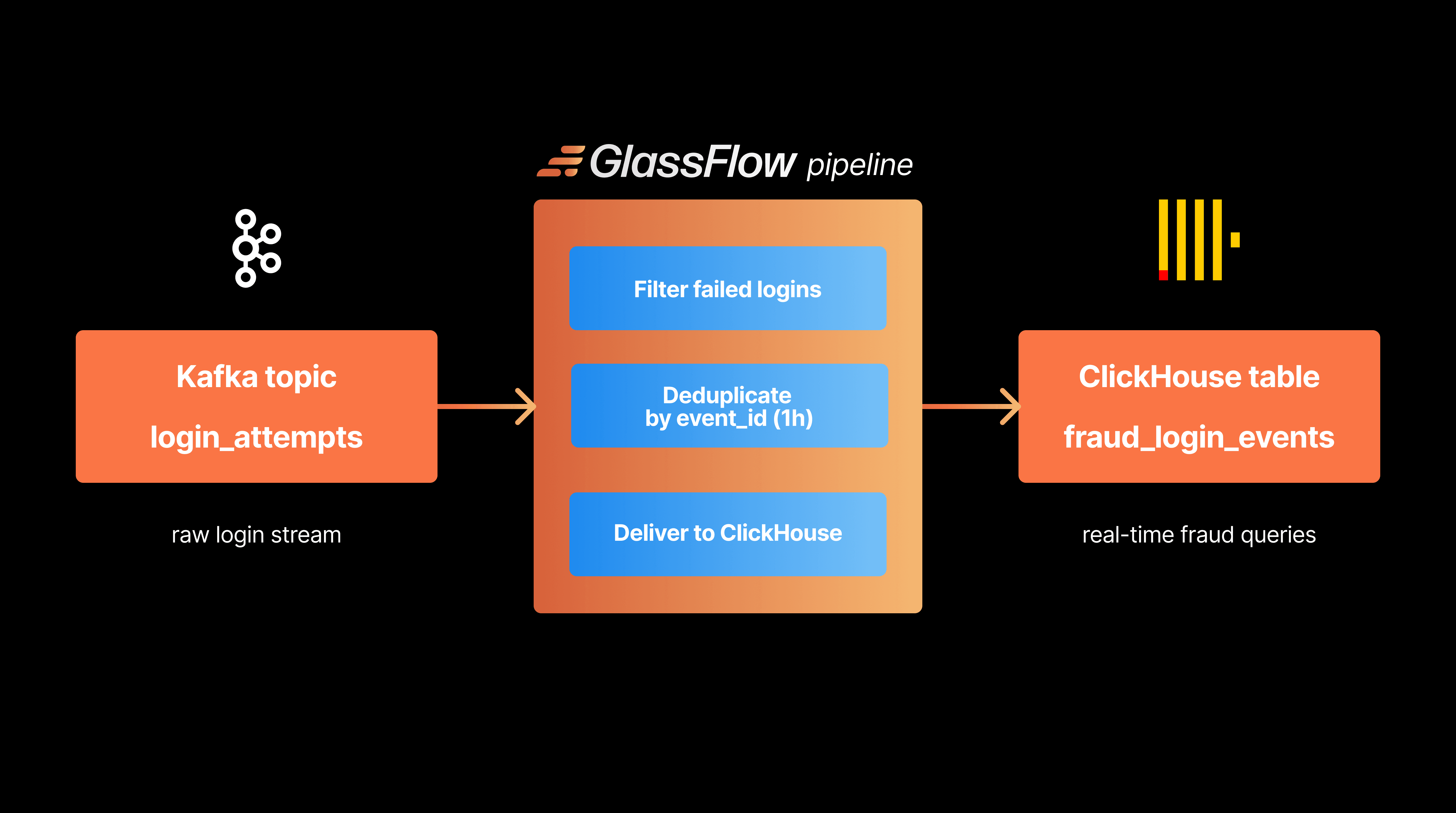


Data transformations at TB scale for ClickHouse
Get query ready data, lower ClickHouse load, and reliable pipelines at enterprise scale.
